This is based on code from the following book
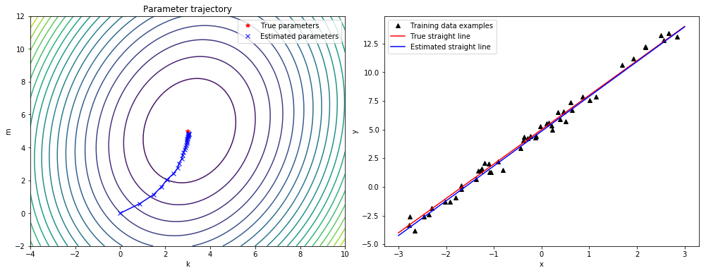
The follow blog post walks through what Parameter Estimation is. The goal here is to explain the theory. I have rewritten this notebook from the above book’s PyTorch Tensor implementation to be just in pure Numpy.
Link to Jupyter Notebook that this blog post was made from
The story here is we’ll learn about Parameter Estimation by pretending we have two thermometers on our desk. One we know measures in Celsius and the other is in a unit we don’t know, hint its Fahrenheit. Our goal is to create a simple model to take a measurement from the unknown thermometer and predict a measurement in Celsius.
Importing required libraries
%matplotlib inline
import numpy as np
import torch
torch.set_printoptions(edgeitems=2, linewidth=75)
Creating our input data
t_c = [0.5,  14.0, 15.0, 28.0, 11.0,  8.0,  3.0, -4.0,  6.0, 13.0, 21.0]
t_u = [35.7, 55.9, 58.2, 81.9, 56.3, 48.9, 33.9, 21.8, 48.4, 60.4, 68.4]
t_c = torch.tensor(t_c)
t_u = torch.tensor(t_u)
Defining our simple linear regression model
def model(t_u, w, b):
    return w * t_u + b
Defining our mean squared error loss function
def loss_fn(t_p, t_c):
    squared_diffs = (t_p - t_c)**2
    return squared_diffs.mean()
Initializing our betas and make our first prediction. This is understandably going to be garbage as our betas are just ones and zeros to be initialized and our starting points for learning.
w = torch.ones(())
b = torch.zeros(())

t_p = model(t_u, w, b)
t_p
tensor([35.7000, 55.9000, 58.2000, 81.9000, 56.3000, 48.9000, 33.9000,
        21.8000, 48.4000, 60.4000, 68.4000])
Compute the loss which we expect to be high, due to the terrible betas.
loss = loss_fn(t_p, t_c)
loss
tensor(1763.8846)
Showing how torch shapes work with multiplication
x = torch.ones(())
y = torch.ones(3,1)
z = torch.ones(1,3)
a = torch.ones(2, 1, 1)
print(f"shapes: x: {x.shape}, y: {y.shape}")
print(f"        z: {z.shape}, a: {a.shape}")
print("x * y:", (x * y).shape)
print("y * z:", (y * z).shape)
print("y * z * a:", (y * z * a).shape)
shapes: x: torch.Size([]), y: torch.Size([3, 1])
        z: torch.Size([1, 3]), a: torch.Size([2, 1, 1])
x * y: torch.Size([3, 1])
y * z: torch.Size([3, 3])
y * z * a: torch.Size([2, 3, 3])
Demonstrates how big our steps would be when adjusting our biases if we did not use a learning_rate hyper parameter.
delta = 0.1

loss_rate_of_change_w = \
    (loss_fn(model(t_u, w + delta, b), t_c) -
     loss_fn(model(t_u, w - delta, b), t_c)) / (2.0 * delta)
loss_rate_of_change_w
tensor(4517.2979)
Demonstrates how the steps are made smaller by a small learning_rate
learning_rate = 1e-2

w = w - learning_rate * loss_rate_of_change_w
w
tensor(-44.1730)
loss_rate_of_change_b = \
    (loss_fn(model(t_u, w, b + delta), t_c) -
     loss_fn(model(t_u, w, b - delta), t_c)) / (2.0 * delta)

b = b - learning_rate * loss_rate_of_change_b
b
tensor(46.0250)
derivative of our loss function
def dloss_fn(t_p, t_c):
    dsq_diffs = 2 * (t_p - t_c) / t_p.size(0)  # <1>
    return dsq_diffs
derivative of model w.r.t w
def dmodel_dw(t_u, w, b):
    return t_u
derivative of model w.r.t b
def dmodel_db(t_u, w, b):
    return 1.0
TODO why dloss_dtp * ...
def grad_fn(t_u, t_c, t_p, w, b):
    dloss_dtp = dloss_fn(t_p, t_c)
    dloss_dw = dloss_dtp * dmodel_dw(t_u, w, b)
    dloss_db = dloss_dtp * dmodel_db(t_u, w, b)
    return torch.stack([dloss_dw.sum(), dloss_db.sum()])  # <1>
def training_loop(n_epochs, learning_rate, params, t_u, t_c):
    for epoch in range(1, n_epochs + 1):
        w, b = params

        t_p = model(t_u, w, b)  # <1>
        loss = loss_fn(t_p, t_c)
        grad = grad_fn(t_u, t_c, t_p, w, b)  # <2>

        params = params - learning_rate * grad

        print('Epoch %d, Loss %f' % (epoch, float(loss))) # <3>

    return params
This training has no early stopping and the loss will grow indefinitely.
training_loop(
    n_epochs = 100,
    learning_rate = 1e-2,
    params = torch.tensor([1.0, 0.0]),
    t_u = t_u,
    t_c = t_c)
Epoch 1, Loss 1763.884644
Epoch 2, Loss 5802485.500000
Epoch 3, Loss 19408035840.000000
Epoch 4, Loss 64915909902336.000000
Epoch 5, Loss 217130559820791808.000000
Epoch 6, Loss 726257583152928129024.000000
Epoch 7, Loss 2429183992928415200051200.000000
Epoch 8, Loss 8125126681682403942989824000.000000
Epoch 9, Loss 27176891792249147543971428302848.000000
Epoch 10, Loss 90901154706620645225508955521810432.000000
Epoch 11, Loss inf
Epoch 12, Loss inf
Epoch 13, Loss inf
Epoch 14, Loss inf
Epoch 15, Loss inf
Epoch 16, Loss inf
Epoch 17, Loss inf
Epoch 18, Loss inf
Epoch 19, Loss inf
Epoch 20, Loss inf
Epoch 21, Loss inf
Epoch 22, Loss inf
Epoch 23, Loss nan
Epoch 24, Loss nan
Epoch 25, Loss nan
Epoch 26, Loss nan
Epoch 27, Loss nan
Epoch 28, Loss nan
Epoch 29, Loss nan
Epoch 30, Loss nan
Epoch 31, Loss nan
Epoch 32, Loss nan
Epoch 33, Loss nan
Epoch 34, Loss nan
Epoch 35, Loss nan
Epoch 36, Loss nan
Epoch 37, Loss nan
Epoch 38, Loss nan
Epoch 39, Loss nan
Epoch 40, Loss nan
Epoch 41, Loss nan
Epoch 42, Loss nan
Epoch 43, Loss nan
Epoch 44, Loss nan
Epoch 45, Loss nan
Epoch 46, Loss nan
Epoch 47, Loss nan
Epoch 48, Loss nan
Epoch 49, Loss nan
Epoch 50, Loss nan
Epoch 51, Loss nan
Epoch 52, Loss nan
Epoch 53, Loss nan
Epoch 54, Loss nan
Epoch 55, Loss nan
Epoch 56, Loss nan
Epoch 57, Loss nan
Epoch 58, Loss nan
Epoch 59, Loss nan
Epoch 60, Loss nan
Epoch 61, Loss nan
Epoch 62, Loss nan
Epoch 63, Loss nan
Epoch 64, Loss nan
Epoch 65, Loss nan
Epoch 66, Loss nan
Epoch 67, Loss nan
Epoch 68, Loss nan
Epoch 69, Loss nan
Epoch 70, Loss nan
Epoch 71, Loss nan
Epoch 72, Loss nan
Epoch 73, Loss nan
Epoch 74, Loss nan
Epoch 75, Loss nan
Epoch 76, Loss nan
Epoch 77, Loss nan
Epoch 78, Loss nan
Epoch 79, Loss nan
Epoch 80, Loss nan
Epoch 81, Loss nan
Epoch 82, Loss nan
Epoch 83, Loss nan
Epoch 84, Loss nan
Epoch 85, Loss nan
Epoch 86, Loss nan
Epoch 87, Loss nan
Epoch 88, Loss nan
Epoch 89, Loss nan
Epoch 90, Loss nan
Epoch 91, Loss nan
Epoch 92, Loss nan
Epoch 93, Loss nan
Epoch 94, Loss nan
Epoch 95, Loss nan
Epoch 96, Loss nan
Epoch 97, Loss nan
Epoch 98, Loss nan
Epoch 99, Loss nan
Epoch 100, Loss nan


tensor([nan, nan])
def training_loop(n_epochs, learning_rate, params, t_u, t_c,
                  print_params=True):
    for epoch in range(1, n_epochs + 1):
        w, b = params

        t_p = model(t_u, w, b)  # <1>
        loss = loss_fn(t_p, t_c)
        grad = grad_fn(t_u, t_c, t_p, w, b)  # <2>

        params = params - learning_rate * grad

        if epoch in {1, 2, 3, 10, 11, 99, 100, 4000, 5000}:  # <3>
            print('Epoch %d, Loss %f' % (epoch, float(loss)))
            if print_params:
                print('    Params:', params)
                print('    Grad:  ', grad)
        if epoch in {4, 12, 101}:
            print('...')

        if not torch.isfinite(loss).all():
            break  # <3>

    return params
training_loop(
    n_epochs = 100,
    learning_rate = 1e-2,
    params = torch.tensor([1.0, 0.0]),
    t_u = t_u,
    t_c = t_c)
Epoch 1, Loss 1763.884644
    Params: tensor([-44.1730,  -0.8260])
    Grad:   tensor([4517.2969,   82.6000])
Epoch 2, Loss 5802485.500000
    Params: tensor([2568.4014,   45.1637])
    Grad:   tensor([-261257.4219,   -4598.9712])
Epoch 3, Loss 19408035840.000000
    Params: tensor([-148527.7344,   -2616.3933])
    Grad:   tensor([15109614.0000,   266155.7188])
...
Epoch 10, Loss 90901154706620645225508955521810432.000000
    Params: tensor([3.2144e+17, 5.6621e+15])
    Grad:   tensor([-3.2700e+19, -5.7600e+17])
Epoch 11, Loss inf
    Params: tensor([-1.8590e+19, -3.2746e+17])
    Grad:   tensor([1.8912e+21, 3.3313e+19])


tensor([-1.8590e+19, -3.2746e+17])
training_loop(
    n_epochs = 100,
    learning_rate = 1e-4,
    params = torch.tensor([1.0, 0.0]),
    t_u = t_u,
    t_c = t_c)
Epoch 1, Loss 1763.884644
    Params: tensor([ 0.5483, -0.0083])
    Grad:   tensor([4517.2969,   82.6000])
Epoch 2, Loss 323.090546
    Params: tensor([ 0.3623, -0.0118])
    Grad:   tensor([1859.5493,   35.7843])
Epoch 3, Loss 78.929634
    Params: tensor([ 0.2858, -0.0135])
    Grad:   tensor([765.4667,  16.5122])
...
Epoch 10, Loss 29.105242
    Params: tensor([ 0.2324, -0.0166])
    Grad:   tensor([1.4803, 3.0544])
Epoch 11, Loss 29.104168
    Params: tensor([ 0.2323, -0.0169])
    Grad:   tensor([0.5781, 3.0384])
...
Epoch 99, Loss 29.023582
    Params: tensor([ 0.2327, -0.0435])
    Grad:   tensor([-0.0533,  3.0226])
Epoch 100, Loss 29.022669
    Params: tensor([ 0.2327, -0.0438])
    Grad:   tensor([-0.0532,  3.0226])


tensor([ 0.2327, -0.0438])
Scaling our t_un Tensor to be more like t_c. See before:
print(t_u)
print(t_c)
tensor([35.7000, 55.9000, 58.2000, 81.9000, 56.3000, 48.9000, 33.9000,
        21.8000, 48.4000, 60.4000, 68.4000])
tensor([ 0.5000, 14.0000, 15.0000, 28.0000, 11.0000,  8.0000,  3.0000,
        -4.0000,  6.0000, 13.0000, 21.0000])
t_un = 0.1 * t_u
And after:
print(t_un)
print(t_c)
tensor([3.5700, 5.5900, 5.8200, 8.1900, 5.6300, 4.8900, 3.3900, 2.1800,
        4.8400, 6.0400, 6.8400])
tensor([ 0.5000, 14.0000, 15.0000, 28.0000, 11.0000,  8.0000,  3.0000,
        -4.0000,  6.0000, 13.0000, 21.0000])
training_loop(
    n_epochs = 100,
    learning_rate = 1e-2,
    params = torch.tensor([1.0, 0.0]),
    t_u = t_un, # <1>
    t_c = t_c)
Epoch 1, Loss 80.364342
    Params: tensor([1.7761, 0.1064])
    Grad:   tensor([-77.6140, -10.6400])
Epoch 2, Loss 37.574917
    Params: tensor([2.0848, 0.1303])
    Grad:   tensor([-30.8623,  -2.3864])
Epoch 3, Loss 30.871077
    Params: tensor([2.2094, 0.1217])
    Grad:   tensor([-12.4631,   0.8587])
...
Epoch 10, Loss 29.030487
    Params: tensor([ 2.3232, -0.0710])
    Grad:   tensor([-0.5355,  2.9295])
Epoch 11, Loss 28.941875
    Params: tensor([ 2.3284, -0.1003])
    Grad:   tensor([-0.5240,  2.9264])
...
Epoch 99, Loss 22.214186
    Params: tensor([ 2.7508, -2.4910])
    Grad:   tensor([-0.4453,  2.5208])
Epoch 100, Loss 22.148710
    Params: tensor([ 2.7553, -2.5162])
    Grad:   tensor([-0.4446,  2.5165])


tensor([ 2.7553, -2.5162])
params = training_loop(
    n_epochs = 5000,
    learning_rate = 1e-2,
    params = torch.tensor([1.0, 0.0]),
    t_u = t_un,
    t_c = t_c,
    print_params = False)

params
Epoch 1, Loss 80.364342
Epoch 2, Loss 37.574917
Epoch 3, Loss 30.871077
...
Epoch 10, Loss 29.030487
Epoch 11, Loss 28.941875
...
Epoch 99, Loss 22.214186
Epoch 100, Loss 22.148710
...
Epoch 4000, Loss 2.927680
Epoch 5000, Loss 2.927648


tensor([  5.3671, -17.3012])
%matplotlib inline
from matplotlib import pyplot as plt
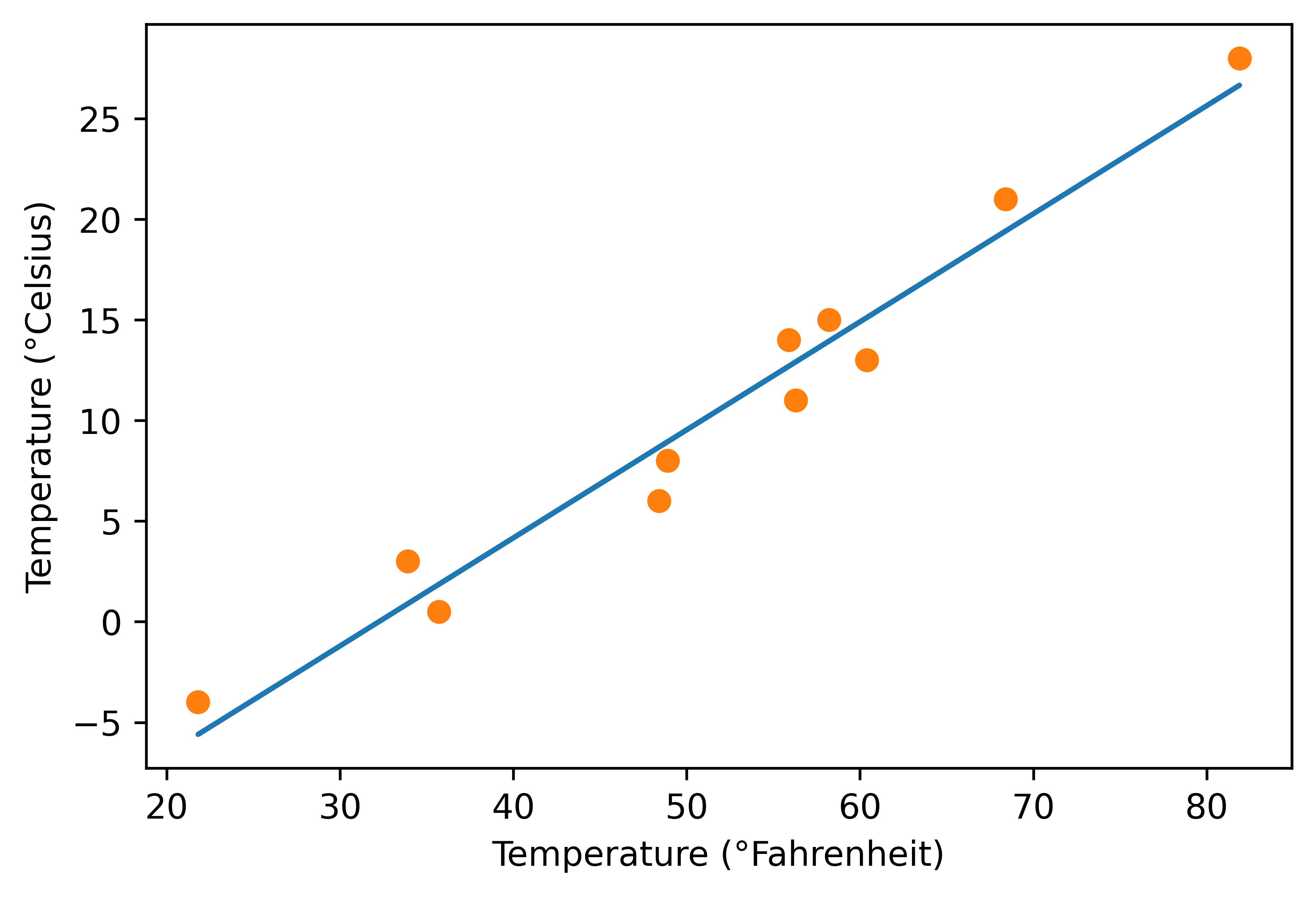
t_p = model(t_un, *params) # <1>
fig = plt.figure(dpi=600)
plt.xlabel("Temperature (°Fahrenheit)")
plt.ylabel("Temperature (°Celsius)")
plt.plot(t_u.numpy(), t_p.detach().numpy()) # <2>
plt.plot(t_u.numpy(), t_c.numpy(), 'o')
plt.savefig("temp_unknown_plot.png", format="png") # bookskip
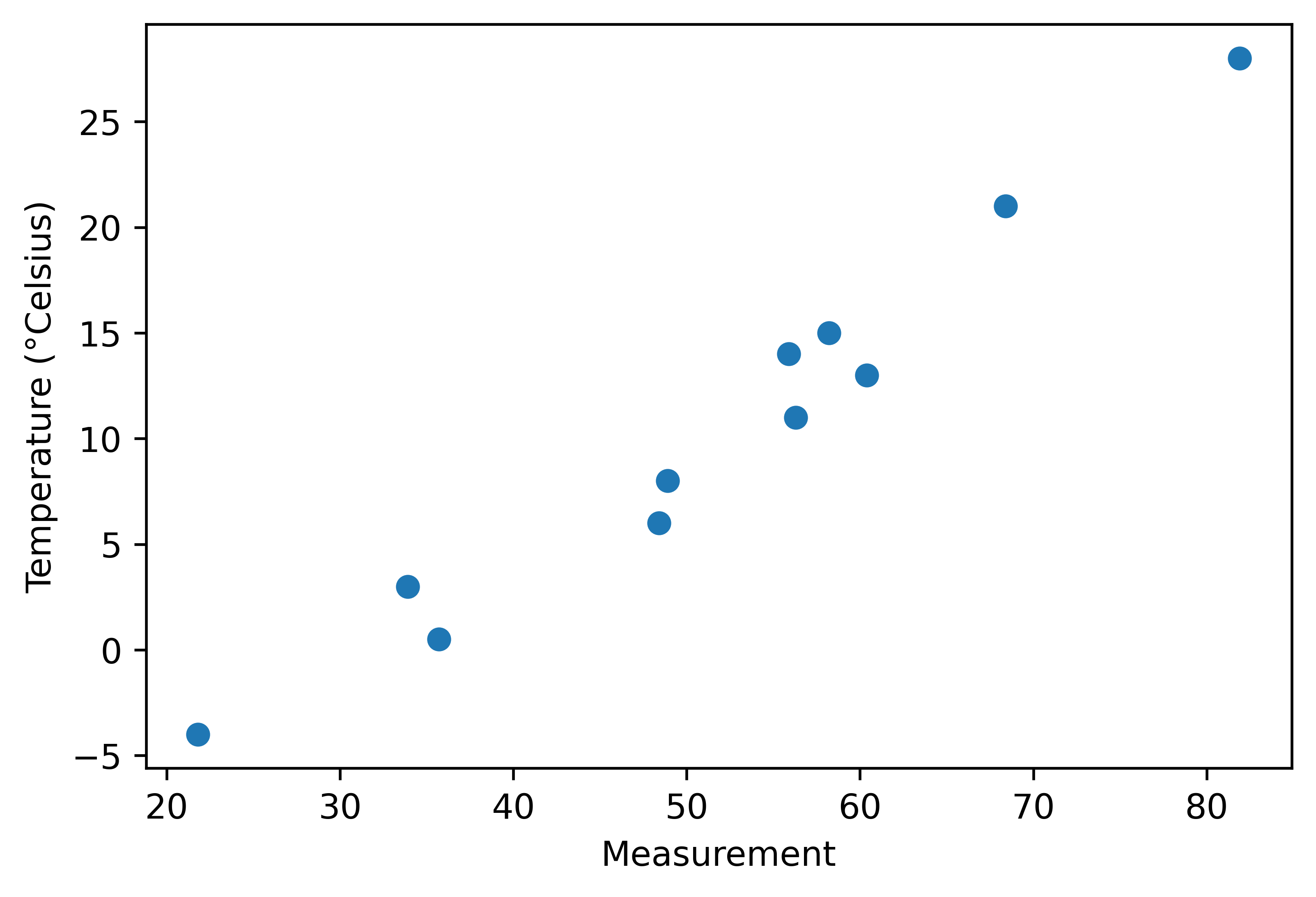
%matplotlib inline
from matplotlib import pyplot as plt

fig = plt.figure(dpi=600)
plt.xlabel("Measurement")
plt.ylabel("Temperature (°Celsius)")
plt.plot(t_u.numpy(), t_c.numpy(), 'o')

plt.savefig("temp_data_plot.png", format="png")
If anything is unclear, please post a comment below!