
Goal Of This “Data Science From Scratch To Production MVP Style” Series?
The goal of this series is to walk through four steps:
- Create a pipeline to process raw data
- Create a simple model to make predictions on future raw data
- Wrap the pipeline and model in a simple API
- Deploy the API to production, using AWS Lambda
Each step above will have its own blog post. This is the first of the four.
Introduction
Let’s pretend that we’re approached by a local ice cream shop owner and asked to start a new project from scratch. The owner has a set of data from his store in Europe and he would like us to:
- Process the European style data into a more “American friendly” format
- Create a simple model to predict ice cream sales
- Wrap our work in an API that’s publicly accessible
The owner makes special emphasis that our approach should very much be a “minimum viable product”.
import dill
import numpy as np
import pandas as pd
import seaborn as sns

from matplotlib import pyplot
from sklearn.base import BaseEstimator, TransformerMixin
from sklearn.linear_model import LinearRegression
from sklearn.model_selection import train_test_split
from sklearn.pipeline import make_pipeline, FeatureUnion, _fit_transform_one, _transform_one
Data Injestion
We’ll just create a Pandas Data Frame from the csv the owner gave us. If you’d like to learn move about how this mock data was generated, read here
df = pd.read_csv("ice_cream_shop.csv", index_col=0)
Data Exploration
Lets take a look at a few rows from the data set before we brainstorm our approach.
df.head()
| temperature_celsius | ice_cream_sales_euro | |
|---|---|---|
| 2019-04-09 | 2.086107 | 49760.279205 |
| 2019-04-10 | 1.807798 | 27942.939525 |
| 2019-04-11 | 2.844184 | 36296.046154 |
| 2019-04-12 | 2.782664 | 41934.780404 |
| 2019-04-13 | 1.090645 | 21253.228606 |
The first takeaway one should have is
This ice cream shop owner has access to a very expensive thermometer
Past that, we see that this data is is very simple, with only three columns a 365 rows.
Looking at the table, we can identify a few cleaning steps we’ll perform together:
- limit
temperature_celsiusto two decimal places, rounding up - convert
temperature_celsiusto fahrenheit
We can also graph a scatter plot using our single independent variable (temperature_celsius) and or single
dependent variable (ice_cream_sales_euro)
sns.set(font_scale=1.8)

a4_dims = (15, 10)
fig, ax = pyplot.subplots(figsize=a4_dims)
sns.regplot(x="temperature_celsius", y="ice_cream_sales_euro", data=df).set_title("Scatter Plot Our Only Independent Variable Against Our Only Dependent Variable")
fig.savefig("regplot.png")
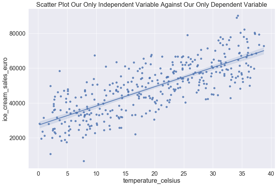
We can see above that there looks to clearly be a linear relation between temperature_celsius and
ice_cream_sales_euro.
For simplicity, we’ll plan on using a linear regression model to predict.
This should satisfy the owner’s request to make the data more “American friendly”.
Pipeline
Generally there are different levels of quality you’ll find in notebooks with regards to pipelining:
- lines of code are written and use the notebook to execute.
- functions are written and then those are called
Today, we’re going to go yet another step further than that leverage scikit-learn’s pipeline.
What’s wonderful about scikit-learn’s pipeline is that the flow respects directed acyclic graphs which means you can process things in parallel or have steps wait for other steps to finish. Additionally, the pipeline will be agnostic to the data you bind it to, meaning once you’re done you can package up the finished pipeline object it and apply it to any other dataset that has the same rows.
This will require us to write a class for each step in our pipeline, where each class extends BaseEstimator and
TransformerMixin. Important things to note:
- our
__init__method is not for passing our data sets in, but rather configurations- rather, the data should be passsed into
fit_transformwhich is just a handy wrapper for callingfitand thentransform
- rather, the data should be passsed into
- We inherit
get_paramsandset_paramsfromBaseEstimator- no need to override these
- the
fitmethod is where we- check parameters
- calculate and add new variables
- return
selffor further scikit-learn compatibility
- the
transformmethod is where we- perform all logic
- return our modified column
For more information feel free to read this excellent blog post
To acheive this, we’ll write agnostic generic steps that will take in columns. By writing it this way, we can augment how we want to leverage this code when we call it, making it more reusuable.
limit temperature_celsius and ice_cream_sales_usd to two decimal places, rounding up
class DecimalRounder(BaseEstimator, TransformerMixin):
    def __init__(self, columns, nth_decimal):
        self.columns = columns
        self.nth_decimal = nth_decimal

    def fit(self, X, y = None):
        assert isinstance(X, pd.DataFrame)

        return self

    def transform(self, X, y = None):
        for column in self.columns:
            X.loc[:,column] = X[column].apply(lambda row: round(row, self.nth_decimal))

        return X
convert temperature_celsius to fahrenheit
class CelciusToFahrenheitCoverter(BaseEstimator, TransformerMixin):
    def __init__(self, columns, new_columns):
        self.columns = columns
        self.new_columns = new_columns

    def fit(self, X, y = None):
        assert isinstance(X, pd.DataFrame)

        return self

    def transform(self, X, y = None):
        for column, new_column in zip(self.columns, self.new_columns):
            X.loc[:,new_column] = X[column].apply(lambda row: row * 9/5 + 32)

        return X
convert ice_cream_sales_euro to US dollars
class ConvertEuroToUsd(BaseEstimator, TransformerMixin):
    def __init__(self, columns, new_columns):
        self.columns = columns
        self.new_columns = new_columns

    def fit(self, X, y = None):
        assert isinstance(X, pd.DataFrame)

        return self

    def transform(self, X, y = None):
        usd_per_euro = 1.09  # at the time of writing this
        for column, new_column in zip(self.columns, self.new_columns):
            X.loc[:,new_column] = X[column].apply(lambda row: row * usd_per_euro)

        return X
Select only specific columns
class FeatureSelector(BaseEstimator, TransformerMixin):
    def __init__(self, columns):
        self.columns = columns

    def fit(self, X, y = None):
        assert isinstance(X, pd.DataFrame)

        return self

    def transform(self, X, y = None):
        return X[self.columns]
Configuring our pipeline
Now this is where the beauty of pipeline comes into play. We get to decide what to pass into our steps and configure it any way we wish. Notice how we could round to three decimal places by not changing any of the pipelining code, only by calling DecimalRounder differently.
pipe = make_pipeline(
            DecimalRounder(["temperature_celsius", "ice_cream_sales_usd"], 2),
            CelciusToFahrenheitCoverter(["temperature_celsius"], ["temperature_fahrenheight"]),
            ConvertEuroToUsd(["ice_cream_sales_euro"], ["ice_cream_sales_usd"]),
            FeatureSelector(["temperature_fahrenheight"])
)
We realize after making our pipeline that we have processed our dependent variable ice_cream_sales_euro, which won’t obviously be available for future predictions on new data. Fortunately, one of the benefits of using scikit-learn’s pipeline is how modular the system is. Lets create a new pipeline that correctly only processes our independent variable temperature_celsius
pipe = make_pipeline(
            DecimalRounder(["temperature_celsius"], 2),
            CelciusToFahrenheitCoverter(["temperature_celsius"], ["temperature_fahrenheight"]),
            FeatureSelector(["temperature_fahrenheight"])
)
Now our pipeline is just processing the independent variable. Notice we haven’t actually executed the pipeline, we’ve just configured how we’ll run it.
Using our pipeline
Now that we have the pipeline steps written and we configured how we’ll call each step, lets actually pass our data through the configured pipeline object.
X = pipe.fit_transform(df)
y = pd.Series(df["ice_cream_sales_euro"].values)
X
| temperature_fahrenheight | |
|---|---|
| 2019-04-09 | 35.762 |
| 2019-04-10 | 35.258 |
| 2019-04-11 | 37.112 |
| 2019-04-12 | 37.004 |
| 2019-04-13 | 33.962 |
| ... | ... |
| 2020-04-03 | 97.322 |
| 2020-04-04 | 98.960 |
| 2020-04-05 | 97.682 |
| 2020-04-06 | 98.888 |
| 2020-04-07 | 97.088 |
365 rows × 1 columns