Big O Notation Explained

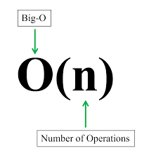
Definition

Big O Notation is a concept often brought up in computer science and is an important thing to consider when designing algorithms. It was created as a way to discuss how many steps an algorithm has to take, regardless of how fast of a computer it was being executed on. In other words, its hardware agnostic. A formal definition for this concept is:

a mathematical notation that describes the limiting behavior of a function when the argument tends towards a particular value or infinity ¹

If I were to reword the above in my own words, I’d say:

a math equation that describes how long an algorithm takes to execute, as its input length grows

I’d like to point out the last part of my summary, as its the most important part and easily the most confusing.

as its input length grows

Big O Notation does not concern itself with what the input to the algorithm is, rather just how many elements are being passed in. The number of elements in your input is referred to as n.

Bounding

Big O Notation is one of the three ways we can bound an algorithm. A specific definition of this is:

We use big-O notation for asymptotic upper bounds, since it bounds the growth of the running time from above for large enough input sizes ²

If I were to reword the above in my own words, I’d say:

Big O Notation defines the worst execution case for a given input length

There are two other notations used, big Ө (read Theta) and big Ω (read Omega) which are responsible for asymptotic tight bound and asymptotic lower bound respectively. These are not used often and for that reason we won’t address them any further.

Calculating Big O

The following is important to note that when you’re calculating Big O:

If f(x) is a sum of several terms, if there is one with largest growth rate, it can be kept, and all others omitted ³

If f(x) is a product of several factors, any constants (terms in the product that do not depend on x) can be omitted. ³

An example of the above statements would be:

1. O(10 + 5n) => O(n)

   We’d drop the constants 10 and 5.

2. O(n + n^2) => O(n^2)

   We’d keep the largest growth rate.

Examples

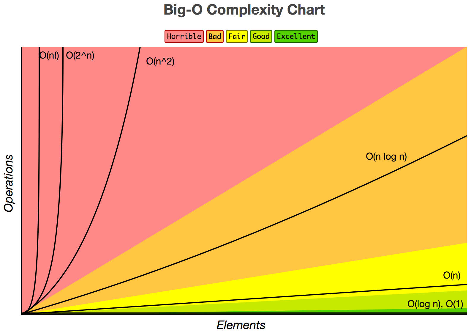
To calculate Big O of an algorithm, you’re generally looking at how many times your code loops, based on the input length. Lets list the common complexities and then provide an example for each one either with code or explanations. The common time complexities are listed in increasing time.

Please note, what is considered a “fast” solution all depends on what problem you’re trying to solve. Some problems’ best solutions are current O(c^n). There might be better solutions out there, but none have been found. To get a better understanding about how these times compare, I find it easier to look at the above equations graphically:

O(1) Constant

The algorithm takes the same amount of time, regardless of the length of the input. If we had a function called getFirstElementOfList that took in a list of Ints and returned the first one, it would take the same time to execute, regardless of the length of the list.

 1
 2
 3
 4
 5
 6
 7
 8
 9
10
11
12
13

func getFirstElementOfList(list: [Int]) -> Int {
  var steps = 0;

  steps += 1

  print("n (input length): \(list.count), steps: \(steps)")

  return list[0]
}

getFirstElementOfList(list: [1])     // n (input length): 1, steps: 1
getFirstElementOfList(list: [1, 2])  // n (input length): 2, steps: 1
getFirstElementOfList(list: [1, 3])  // n (input length): 3, steps: 1

The important component is the prints above, you can see that the steps our algorithm takes is always O(1), which is the worst case. This is called a constant algorithm, as it takes a constant amount of steps regardless of the size n and is the fastest time complexity that can be achieved.

O(log(n)) Logarithmic

This time complexity might be a little difficult to understand at first, but its fairly simple once you remember that the log function is the opposite of the exponential function. So an algorithm with the time complexity of log(n) will be halving the number of data points it will be looking at, at each step. A common example of this is searching through a balanced binary search tree. Lets look at an image to explain this, as the code to show this would be longer than the other examples:

⁴

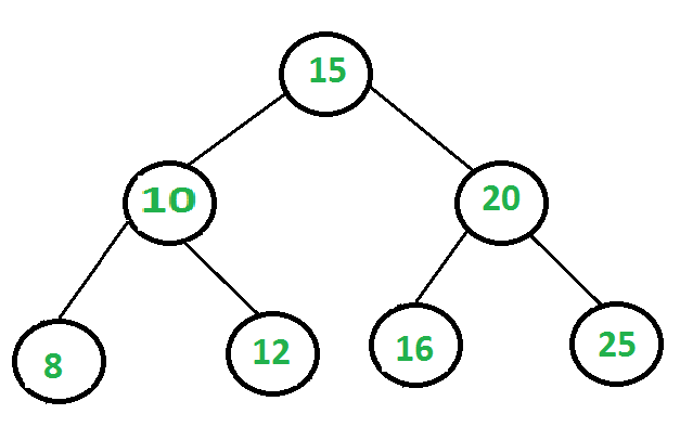
If we were to search the above tree for the number 12, we’d take the following steps:

1. Initial Step:

   Possible Numbers Left To Evaluate = 7

2. Evaluate 15: This is not the number we are looking for (12) and our target number (12) is less than this, so we go left

   Possible Numbers Left To Evaluate = 3

3. Evaluate 10: This is not the number we are looking for (12) and our target number (12) is more than this, so we go right

   Possible Numbers Left To Evaluate = 1

4. Evaluate 12: This is the number we are looking for

   Possible Numbers Left To Evaluate = 0

You can see that at each step we halved the amount of numbers left to evaluate. This is a logarithmic function, using the log base two operation.

Searching through seven nodes in the binary search tree only took three steps. If we were to do this example with various amounts of nodes, the number of steps would look like:

We can see that the number of steps does increase with n, but at a very slow rate. I suggest looking up at the colorful chart to get a good sense at how slow O(log(n)) really does grow.

O(n) Linear

An algorithm with O(n) time means that each element in the input list must be visited once to solve the problem. Lets say we wanted to sum every value in the list, this task would require us to look at every element so we could add it to the running total. There would be no way to solve this problem by ignoring one or more elements, which is why the time complexity is called linear, as it grows at the same rate of the input size does.

 1
 2
 3
 4
 5
 6
 7
 8
 9
10
11
12
13
14
15
16
17

func sumNumbers(list: [Int]) -> Int {
  var steps = 0
  var sum = 0

  for element in list {
    sum += element
    steps += 1
  }

  print("n (input length): \(list.count), steps: \(steps)")

  return sum
}

sumNumbers(list: [1])       // n (input length): 1, steps: 1
sumNumbers(list: [1, 2])    // n (input length): 2, steps: 2
sumNumbers(list: [1, 2, 3]) // n (input length): 3, steps: 3

The important component is the prints above, you can see that the steps our algorithm takes is always O(n), which is the worst case.

O(n^2) Quadratic

An algorithm with O(n^2) time means we’ll visit every element in the data set n times, at most. A classic example of this time complexity is Bubble Sort, which is an easy sort to follow but performs very poorly. How it essentially works is by looping at each number in the list at a time (called i in our code example), and then comparing that to every other number in the list (called j in our code example).

 1
 2
 3
 4
 5
 6
 7
 8
 9
10
11
12
13
14
15
16
17
18
19
20
21
22
23
24

func bubbleSort(unsortedList: [Int]) -> [Int] {
  var steps = 0
  var sortedList = unsortedList

  for (i, _) in sortedList.enumerated() {
    for (j, _) in sortedList.enumerated() {
      if sortedList[i] < sortedList[j] {
        let temp = sortedList[i]
        sortedList[i] = sortedList[j]
        sortedList[j] = temp
      }

      steps += 1
    }
  }

  print("n (input length): \(unsortedList.count), steps: \(steps)")

  return sortedList
}

bubbleSort(unsortedList: [2, 1])         // n (input length): 2, steps:  4
bubbleSort(unsortedList: [3, 2, 1])      // n (input length): 3, steps:  9
bubbleSort(unsortedList: [4, 3, 2, 1])   // n (input length): 4, steps: 16

The important component is the prints above, you can see that the steps our algorithm takes is always O(n^2), which is the worst case.

O(n^c) Polynomial

Note: Usually c is 2.

A polynomial is slowest time complexity that is still considered to be fast. Note that we are raising n to some constant c, which means as n grows, the portion of our equation responsible for the most increase is still c, which is a constant. So the growth should be rather slow.

An example of a polynomial function is Selection Sort.

 1
 2
 3
 4
 5
 6
 7
 8
 9
10
11
12
13
14
15
16
17
18
19
20
21
22
23
24
25
26
27
28
29
30
31
32
33
34
35

func selectionSort(_ unsortedArray: [Int]) -> [Int] {
    guard unsortedArray.count > 1 else { return unsortedArray }

    var steps = 0
    var sortedArray = unsortedArray

    for x in 0 ..< sortedArray.count - 1 {
        var lowest = x

        for y in x + 1 ..< sortedArray.count {
            if sortedArray[y] < sortedArray[lowest] {
                lowest = y
            }

            steps += 1
        }

        if x != lowest {
            sortedArray.swapAt(x, lowest)
        }
    }

    print("n (input length): \(unsortedArray.count), steps: \(steps)")
    return sortedArray
}

selectionSort([2, 1])                           // n (input length):  2, steps:  1
selectionSort([3, 2, 1])                        // n (input length):  3, steps:  3
selectionSort([4, 3, 2, 1])                     // n (input length):  4, steps:  6
selectionSort([5, 4, 3, 2, 1])                  // n (input length):  5, steps: 10
selectionSort([6, 5, 4, 3, 2, 1])               // n (input length):  6, steps: 15
selectionSort([7, 6, 5, 4, 3, 2, 1])            // n (input length):  7, steps: 21
selectionSort([8, 7, 6, 5, 4, 3, 2, 1])         // n (input length):  8, steps: 28
selectionSort([9, 8, 7, 6, 5, 4, 3, 2, 1])      // n (input length):  9, steps: 36
selectionSort([10, 9, 8, 7, 6, 5, 4, 3, 2, 1])  // n (input length): 10, steps: 45

Note: Usually c is 2.

We see above that as n grows, so does the number of steps, at an increasing rate. This is a property of the polynomial time. We’ll see the same thing, but at a much faster rate in our next time complexity.

You might be thinking, why aren’t the number of steps as big as n^c, and that’s because these are worst case. So in practice above, we did not reach the worst case scenario, but it is possible to do so.

O(c^n) Exponential

An exponential time complexity is the worst speed we’ll discuss today. Not only does the number of steps increase as the input length n increase, but the rate that it increases does so incredibly quickly. Lets look at a simple example that adds one to a running some for every step it takes:

 1
 2
 3
 4
 5
 6
 7
 8
 9
10
11
12
13
14
15
16
17
18
19
20
21
22

import Foundation

func dumbExponentialAddititon(_ array: [Int]) {
    var steps = 0
    var someConstant:Decimal = 2.0
    var numberOfTimesToIterate = Int(NSDecimalNumber(decimal: pow(someConstant, array.count)))

    for i in 1...numberOfTimesToIterate {
        steps += 1
    }

    print("n (input length): \(array.count), steps: \(steps)")
}

dumbExponentialAddititon([3, 2, 1])                        // prints n (input length):  3, steps:    8
dumbExponentialAddititon([4, 3, 2, 1])                     // prints n (input length):  4, steps:   16
dumbExponentialAddititon([5, 4, 3, 2, 1])                  // prints n (input length):  5, steps:   32
dumbExponentialAddititon([6, 5, 4, 3, 2, 1])               // prints n (input length):  6, steps:   64
dumbExponentialAddititon([7, 6, 5, 4, 3, 2, 1])            // prints n (input length):  7, steps:  128
dumbExponentialAddititon([8, 7, 6, 5, 4, 3, 2, 1])         // prints n (input length):  8, steps:  256
dumbExponentialAddititon([9, 8, 7, 6, 5, 4, 3, 2, 1])      // prints n (input length):  9, steps:  512
dumbExponentialAddititon([10, 9, 8, 7, 6, 5, 4, 3, 2, 1])  // prints n (input length): 10, steps: 1024

Since c was 2, we can see the number of steps required are all powers of 2. Exponential functions should be avoided if quicker alternatives exist, but many problems do not have solutions that are faster than exponential time, or at least they haven’t been discovered/invented yet. Some famous problems include evaluating a checkers, chess or go board.

Conclusion

Now you should be familiar with what Big O Notation is and the common time complexities. I’d say that in general, you’ll want to be aware of the time complexity of the algorithm you’re writing and additionally know what kind of data you can expect to be working with. For example, if you’re function will only receive at most ten elements, than spending the time and effort to go from O(n^2) to O(n) might not be worth it.

If I made any mistakes or something is unclear, please reach out to me via any of the social channels above, or leave a comment below. Thank you.

Additional Resources

• Big O Cheat Sheet
• Various Big O Complexity Examples