Digest: A Few Useful Things to Know about Machine Learning

Digest of This paper: A Few Useful Things to Know about Machine Learning

In this digest format, I’ll simply be quoting portions of the paper I found interesting. This is mainly a method for me to summarize papers I’ll be reading, both out of interest and out of hopes at getting better at reading white papers. Comments and questions are appreciated at the bottom. All quotes are from the papers.

Highlights

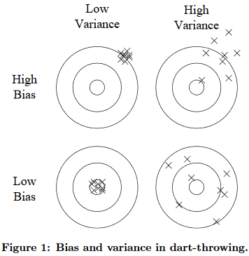
• Bias is a learner’s tendency to consistently learn the same wrong thing. Variance is the tendency to learn random things irrespective of the real signal. Figure 1 illustrates this by an analogy with throwing darts at a board

  • This is an excellent way to explain the bias variance trade off, especially when looking at the graphic. This is just like learning the difference between accuracy and precision, same graphic.

• …decision trees learned on different training sets generated by the same phenomenon are often very different, when in fact they should be the same.

  • This is why random forests are possible, as you end up taking your entire training set and exposing each decision tree to a subset. If every decision tree ended up being the same, a random forest would be a forest of the same trees and provide no benefit.

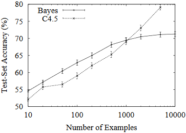
• …contrary to intuition, a more powerful learner is not necessarily better than a less powerful one. Figure 2 illustrates this. Even though the true classifier is a set of rules, with up to 1000 examples naive Bayes is more accurate than a rule learner. This happens despite naive Bayes’s false assumption that the frontier is linear!

  • This is such a great concept and is mentioned a few times throughout the paper. This paper really pushes trying out to simplest model first and seeing where that gets you. The simpler models are usually quicker to get up and running and might produce good enough results.

• “false discovery rate”: falsely accepted non-null hypotheses

• “curse of dimensionality”: many algorithms that work fine in low dimensions become intractable when the input is high-dimensional

• Generalizing correctly becomes exponentially harder as the dimensionality (number of features) of the examples grows, because a fixed-size training set covers a dwindling fraction of the input space. Even with a moderate dimension of 100 and a huge training set of a trillion examples, the latter covers only a fraction of about $10^{-18}$ of the input space.

  • The coverage becomes even smaller when the dimensions represent continuous variables.

• If there are no other features, this is an easy problem. But if there are 98 irrelevant features $x_3$, …, $x_{100}$, the noise from them completely swamps the signal in $x_1$ and $x_2$, and nearest neighbor effectively makes random predictions.

  • This is why “feature selection” is an important concept. You can’t just add random data to your data set and hope that it will have no negative effect. You have to evaluate each and every feature, determining what is worth keeping in.

• Even more disturbing is that nearest neighbor still has a problem even if all 100 features are relevant! This is because in high dimensions all examples look alike.

  • This is a concept I had not considered before. Very neat!

• Naively, one might think that gathering more features never hurts, since at worst they provide no new information about the class. But in fact their benefits may be outweighed by the curse of dimensionality.

  • Again, shows the importance of “feature selection”

• Learners can implicitly take advantage of this lower effective dimension, or algorithms for explicitly reducing the dimensionality can be used

• …bear in mind that features that look irrelevant in isolation may be relevant in combination

  • Keeping this in mind is always time consuming when performing your EDA. Not only do you end up looking at each feature in isolation, but also how the features relate to and perform with others.

• Suppose you’ve constructed the best set of features you can, but the classifiers you’re getting are still not accurate enough. What can you do now? There are two main choices: design a better learning algorithm, or gather more data.

  • This points to the classic situation where every data scientist wants more data.

• As a rule of thumb, a dumb algorithm with lots and lots of data beats a clever one with modest amounts of it.

  • Kind of related to figure 2, but a neat concept to consider. Generally the difference between a dumb and clever algorithm is just how effectively they use the data they have, which boils down to having more data used poorly vs less data used effectively.

• In most of computer science, the two main limited resources are time and memory. In machine learning, there is a third one: training data. Which one is the bottleneck has changed from decade to decade. In the 1980’s it tended to be data. Today it is often time. Enormous mountains of data are available, but there is not enough time to process it, so it goes unused.

  • As someone who comes from a computer science background, its an interesting new twist on how you have to approach problems.

• As a rule, it pays to try the simplest learners first (e.g., naive Bayes before logistic regression, k-nearest neighbor before support vector machines). More sophisticated learners are seductive, but they are usually harder to use, because they have more knobs you need to turn to get good results, and because their internals are more opaque.

  • Finally, the last and my favorite quote. I mentioned this early, but the idea of starting out as simple as possible and iterate, improving if needed, seems like the best approach and usage of one’s time.